The Ordinary Sachs-Wolfe Effect
Given the picture of the universe at recombination that we have just roughly sketched, we might expect that we are able to model the dynamics of this photon-baryon fluid using many of the same equations and relationships that are used for the modeling the dynamics and kinematics of a simple harmonic oscillator (that is, a spring). In fact, this is precisely what is done in practice, although with a bit more complication than is usually involved with an everyday spring.
We have already mentioned the effect of gravity on the photons present in the photon-baryon fluid in the early universe, but what exactly is that effect? This is where we begin to introduce some degree of complication.
A Few General (Relativity) Ideas
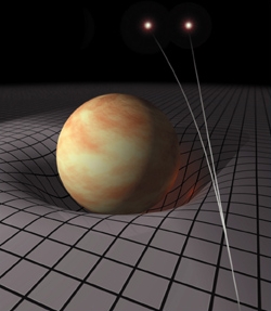
Before we examine the effect of gravity on the photons in the plasma, we must introduce a few ideas. In general relativity (GR), gravity is directly related to the geometry of space. Think of space as consisting of a huge (infinite, even) rubber sheet. Then, a massive body (for our purposes, simply a source of a gravitational potential) sitting in space will create a little dimple on that sheet and effectively curve the space around it, much like the picture to the right (from the cover of Sean Carroll's textbook Spacetime and Geometry). However, what you come to learn in physics is that nothing is perfectly and absolutely smooth. Everything has small fluctuations associated with it such that on average it is smooth, but if you look closely enough you see small fluctuations around that average value.
"The Magic 1/3" (see White and Hu 1997)
As we have already noted, there is an underlying gravitational potential due to the massive particles that do not otherwise interact, the dark matter, in the primordial soup. Thus, we will also have some fluctuation associated with this matter density
Ψ ≡ gravitational potential fluctuation
and we can identify a fluctuation of the gravitational potential as well, and GR also tells us how this is related to Ψ
Φ ≡ curvature fluctuation
Ψ ≈ -Φ
What Sachs and Wolfe worked out in their 1967 paper is that this potential fluctuation introduces a temperature fluctuation into the photons sitting in the photon-baryon fluid that we are then able to measure as we look up at the sky. Their answer, qualitatively, is that the temperature fluctuation is directly related to the gravitational potential fluctuation by some constant. More quantitatively, if we denote

as the intrinsic temperature fluctuation then
![]()
so that the effective temperature Θ+Ψ that arises from solving the combined continuity and Euler equations for the kinematics of the photon-baryon fluid under the influence of gravity becomes
![]()
and hence the "magic 1/3." This is the Sachs-Wolfe effect.
Derivation
To see the origin of this equation, and thus to get our feet wet for the discussion of the integrated Sachs-Wolfe effect, we follow the derivation presented by White and Hu (1997). Beginning with a simple statement of energy conservation, which may be derived from the geodesic equation for photons traveling in a perturbed metric with a curvature perturbation given by Φ we may write

where

is the effective temperature due to both the "intrinsic" temperature perturbation (the first term on the right side) and the effect of the gravitational potential perturbation on the temperature of the photon. If we assume adiabatic temperature fluctuations, which is an assumption greatly favored by the acoustic peak spacing and locations in the WMAP data power spectrum, then a potential well (a low spot in the gravitational potential) will represent an over-density in the photon distribution but a cold spot in the temperature on the sky. If we then consult our favorite GR textbook we realize that the gravitational potential affects the time that a stationary observer will measure. This is an immediate consequence of the spacetime nature of gravity and we find that indeed clocks runs more slowly in a region of curved space than in a region of absolutely flat space (and hence devoid of gravitating bodies and fields). Since we are considering only a fluctuation in the potential (really, the metric) around some average value, we will only concern ourselves with this fluctuation. Moreover, we will consider is to be relatively small. Therefore, we may write this relationship between time and potential as
![]() .
.
We also note that since the expansion of the universe must be taken into account, and since
 ,
,
where w=p/ρ is the equation of state, a later time corresponds to a larger scale factor a and vice versa. What's more, since the universe is cooling off as
![]()
a later time is equivalent to a cooler temperature.
Let's stop to muse over what all of this means. If we focus on just one moment in time we have some average gravitational potential present in the photon-baryon fluid. We also have a fluctuation Φ ≈ -Ψ around this average value. Thus, from the fact that in regions of greater gravitational potential the time coordinate and thus the scale factor is at a smaller value, the temperature is higher. We may thus choose to look at the situation from the perspective that over-densities correspond to later times and under-densities correspond to earlier times. This perspective is illustrated in the diagram below.
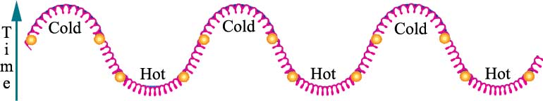
It is somewhat important to note that the fact that I told you that there is a gravitational potential fluctuation is a choice of the time coordinate direction (or more technically, a gauge choice), which is perfectly kosher in GR. From here, we have all of the tools to proceed to the actual derivation of the Sachs-Wolfe effect.
From t α a3(1+w)/2 we have
 ,
,
 ,
,
 .
.
But since we also know that T α a-1 and that the gravitational potential is essentially a perturbation to the time coordinate we have

and
![]()

Combining this with the above relationship

or under the assumption that at the last scattering surface the universe is matter dominated and w=0 (which is not a very good approximation) we have the final answer which gives rise to the "magic 1/3"
![]() .
.
Despite the apparent ease of this derivation compared to the original derivation by Sachs and Wolfe, this is a wholly mathematically rigorous derivation. The key here is the realization that a good choice of constant time surface is not only completely allowable but also eases the complexity of the derivation and improves the ability to intuitively understand the source of the "magic 1/3."
From here, however, we will proceed quickly into the ISW effect and the mathematical description of its predicted contribution to the CMB power spectrum.
•